Voluntary Tax Compliance as a Measurement System: Evidence, Identification, Prediction, and Forecasting

Most tax systems collect most of what they are owed without anybody being audited, prosecuted or even contacted. That fact gets a name, voluntary compliance, and the name is then used as though it referred to something an administration can look up. It does not. A tax administration observes registrations, returns, declared liabilities, payments, arrears, audit adjustments, information mismatches and enforcement actions. It can estimate what should have been paid. It can survey people about legitimacy and willingness. None of those objects is the thing the phrase names.

The gap matters because the same observed outcome can be produced by very different machinery. A high on-time payment rate can come from withholding, from third-party reporting, from prefilled declarations, from a credible belief that non-compliance is detected, from low transaction costs, from intrinsic motivation, or from any mixture of them. The United States Internal Revenue Service projects a voluntary compliance rate of 85.0 per cent for tax year 2022, defined as tax paid voluntarily and on time divided by estimated true tax. That is a coherent accounting definition and it is not a measurement of a psychological propensity, even though the words suggest one.

This note works through what a defensible quantitative programme on this subject actually looks like. It separates four questions that a single administrative dataset can answer and that are routinely collapsed into one number: what the level of compliance is, what causes it to change, which cases are likely to be non-compliant, and what the aggregate indicator will be next year. Measurement models, causal designs, risk scores and forecasts answer those four respectively, and their outputs are not substitutes for one another. Every code block below runs, and the numbers printed under each one came out of running it.

What the phrase denotes, and the four things it is confused with

The most defensible starting point is the four-obligation structure used in tax-administration diagnostics: taxpayers must be appropriately registered, file required declarations on time, report liabilities accurately, and pay what is due on time. Those obligations are separable. A taxpayer can file punctually and under-report, report accurately and pay late, or stay outside the register entirely. The Tax Administration Diagnostic Assessment Tool assesses them through distinct performance dimensions rather than treating compliance as one observed variable.

So the outcome for taxpayer $i$ in period $t$ is a vector, not a scalar:

where $R$, $F$, $A$ and $P$ are registration, filing, accuracy and payment. Even that conceals the denominators. An on-time filing rate needs an estimate of returns expected, not returns received. Registration compliance needs an estimate of the population that ought to be registered. Reporting accuracy cannot normally be observed at all without third-party information, an audit, or a statistical model. Payment compliance depends on the statutory due date and on how instalment plans, disputes, insolvency and later-collected arrears are treated.

Four objects get conflated, and keeping them apart is most of the work.

Obligation outcome indicators are administrative rates: on-time filing, on-time payment. They measure behaviour around one obligation in one time window.

Tax morale is attitudinal. Luttmer and Singhal use the term for the non-pecuniary motivations for paying tax, which can include intrinsic motivation, reciprocity, peer effects, culture and plain misunderstanding. World Values Survey and European Values Study items support cross-national work on attitudes commonly used as proxies. An attitude item is not a tax return.

The tax gap is a monetary counterfactual: what would have arisen under a defined benchmark, minus what was collected or reported. The IMF's RA-GAP methodology further separates the compliance gap from a policy gap that comes from the actual tax system departing from a benchmark structure. A tax gap is therefore not a synonym for deliberate evasion. It absorbs non-filing, mistakes and non-payment, and its size depends on assumptions about the potential base.

Enforced-versus-voluntary decompositions classify receipts by timing or intervention status. The IRS voluntary compliance rate is one: timely voluntary payments over estimated true liability. Psychological instruments such as TAX-I use nearly the same words for a completely different estimand, namely stated voluntary versus enforced motivation. The labels coincide; the constructs do not.

The dashed arrows are the part that is easy to miss. Administrative architecture does not only change behaviour, it changes what is observable. An e-invoicing mandate makes previously invisible under-reporting visible, so the measured gap can rise while behaviour improves. Any inference that reads a movement in the observed column as a movement in the latent box has to rule that out first.

Measurement approaches are not interchangeable

Measurement approach	Primary estimand	Main data requirement	Characteristic failure mode	Cross-country comparability
On-time filing/payment indicator	Share of expected obligations met by the deadline	Register, filing calendar, payment ledger	The denominator depends on how "expected" obligations and "active" taxpayers are defined	Medium, after metadata harmonisation
Top-down VAT gap	Potential VAT liability minus actual VAT revenue	National accounts, supply-use data, statutory rules, receipts	National-accounts error, timing, exemption and rate mapping, and hidden-economy assumptions all land in the residual	Medium within one methodology, weaker across independently produced series
Bottom-up random-audit gap	Population under-reporting inferred from audited sampled units	Probability sample, detailed examinations, sampling weights	Undetected evasion, non-filers and hidden activity need explicit adjustments; the audit itself detects imperfectly	Potentially high if designs are harmonised, which they rarely are
Risk-audit-based gap	Population non-compliance imputed from operational audits	Risk-selected audits plus a selection model	Verification bias: the audited were deliberately not random	Low, without a convincing selection correction
Tax-morale survey	Attitude, norm, or reported willingness to comply	Representative survey with harmonised questions	Social desirability, translation and cultural non-invariance, weak link to behaviour	Medium for harmonised instruments, low for ad hoc ones
Voluntary/enforced accounting split	Share of true liability paid by a point without a specified intervention	Estimated true liability, payments, enforcement records	"Voluntary", "timely" and the enforcement window differ across systems	Low unless definitions and windows are identical
TAX-I-type instrument	Latent voluntary and enforced compliance intentions	Validated survey items	Measures intention, not realised tax behaviour	Medium, with measurement-invariance testing

Top-down and bottom-up gap estimates have no reason to coincide, because they do not start from the same statistical object. A top-down VAT estimate reconstructs potential liability from macroeconomic expenditure or value-added aggregates and maps it through statutory rates and exemptions; the residual absorbs genuine non-compliance and also national-accounts error, timing differences, model approximation and mismatches between economic and legal classifications. IMF methodology describes top-down approaches as deliberately using information independent of tax declarations to build the potential base, which is the whole point and also the whole exposure.

A bottom-up random-audit estimator starts from sampled taxpayers instead. In stylised form,

with $\widehat{G}_{NF}$ for the non-filers and $\widehat{G}_{ND}$ for what an examination fails to detect. The first term is design-consistent under probability sampling if examination reveals true liability. The last two are the difficult ones, and IMF guidance is explicit that adjustments for non-detection, non-payment and activity missing from the filing population are required rather than optional. Risk-selected operational audits are worse again, because the taxpayers in them were chosen precisely for their expected non-compliance.

The IRS National Research Program exists to solve exactly this: its sampling frame represents the filing population rather than the operationally selected subset. HMRC likewise uses random-enquiry data alongside surveys and administrative information for parts of its gap system. Both also demonstrate the cost, since detailed random examinations are expensive and some components still need models.

Published uncertainty is data

HMRC's 2026 edition classifies 35 per cent of its aggregate gap as resting on components with "high" uncertainty and another 14 per cent as "very high". The high share was around 8 per cent in the previous edition. Half the estimate now sits on components its own producers describe as poorly determined, which is not a criticism of HMRC but a reminder that a tax-gap point estimate is not an accounting balance.

The revisions make the same point harder. Here is the same series read from three editions of the same publication:

Tax year	As first published	2026 edition	Change
2021-22	4.8%, later revised to 5.2%	6.0%	+1.2 pp on the revised figure
2022-23	4.8% (£39.8bn, 2024 edition)	6.6%	+1.8 pp
2023-24	5.3% (£46.8bn, 2025 edition)	6.0%	+0.7 pp
2024-25	6.4% (£59.2bn, 2026 edition)	6.4%	first estimate

The 2022-23 tax gap grew by more than a third of its original value without a single taxpayer changing behaviour, because the method changed. Anybody who fitted a model to the 2024 vintage and reported a downward trend was not wrong about the data they had. They were wrong about what the data was.

This has to enter the econometrics rather than the caveats. If a published gap $\widehat g_{ct}$ is a noisy estimate of a latent gap $g_{ct}$,

then a regression that treats $\widehat g_{ct}$ as error-free understates total uncertainty. If the noisy gap is a regressor, classical measurement error attenuates the coefficient. If the measurement error is correlated with administrative capacity, income level or digitalisation, which it certainly is, the bias is not even guaranteed to point towards zero. Carrying $s_{ct}$, or published intervals, or method-specific error parameters into the substantive model is the difference between a hierarchical measurement model and a spreadsheet regression on point estimates.

Reproducible sources, and what "public" means for each

A global project has to separate public documentation from public microdata, because the difference decides whether a result can be independently reproduced or only cited.

Source	Use in compliance research	Access status	Reproducibility
OECD Tax Administration / ISORA tables	Filing, payment, debt, digitalisation, staffing indicators	Publicly accessible portal and tables	Suitable for reproducible cross-country administrative panels, subject to metadata changes and missingness
TADAT performance assessment reports	Standardised diagnostic evidence	Public only where the assessed authority authorises publication	Published reports are reproducible inputs; the universe of assessments is not an open dataset
HMRC Measuring tax gaps	Detailed top-down and bottom-up series with methodology	Publicly downloadable online tables	Good for vintage-aware work, precisely because components get revised
IRS tax gap series	Gross and net gap, voluntary compliance rate	Public aggregates; NRP taxpayer microdata restricted	Aggregate replication possible; independent reproduction of the micro-estimation is not
UNU-WIDER Government Revenue Dataset	Revenue structure and macro-fiscal controls	Open and free	Fully suitable for reproducible macro panels
World Values Survey	Tax-morale and institutional-attitude proxies	Free for non-commercial use after no-charge registration	Reproducible subject to licence and version control
European Values Study	Harmonised values and attitudes	Open, usually through GESIS	Reproducible with the dataset DOI and version recorded
Afrobarometer	Trust, legitimacy and taxation attitudes across Africa	Free to use and download	Useful for attitudes, never for liability
Latinobarómetro	Longitudinal public opinion in Latin America	Public data and documentation download	Harmonised waves support regional attitude panels; archive the licence with the replication materials
World Bank Enterprise Surveys	Firm characteristics and administrative burden	Microdata after registration and a data-access agreement	Replicable by registered users under confidentiality conditions

ISORA's own data tables hold indicators for more than 175 jurisdictions that completed at least one of the five rounds launched between September 2020 and September 2024. Geographic coverage is not measurement equivalence. Cross-country comparison is defensible only after auditing denominators, tax types, fiscal years, filing regimes and methodological breaks, and a panel assembled without that audit produces coefficients about definitional differences rather than about tax.

Why entities comply, and what interventions actually move

The canonical deterrence model is still the right baseline for one mechanism. A taxpayer chooses what to declare under uncertainty, trading the gain from concealment against the probability and consequence of detection. Allingham and Sandmo formalised that in 1972; Yitzhaki then showed that assessing the penalty on evaded tax rather than on concealed income reverses the comparative statics with respect to the tax rate. The theory explains why enforcement probability matters. It predicts almost nothing about where evasion is technically possible, and it cannot explain why people comply when the expected punishment is close to zero.

Information architecture is the strongest empirical addition. Kleven and co-authors audited a stratified, representative sample of over 40,000 Danish income tax filers and found an evasion rate of 0.3 per cent on income subject to third-party reporting against 37 per cent on self-reported income. Because 95 per cent of income in that system is third-party reported, the overall evasion rate is small. That single contrast does more explanatory work than any behavioural parameter: compliance is high where misreporting is arithmetically hard and low where it is easy, in the same country, under the same tax law, among the same people.

Pomeranz showed the same mechanism at firm scale, in two randomised experiments among over 400,000 Chilean firms: VAT paper trails create preventive deterrence, and enforcement spills up the chain to suppliers. Third-party reporting is not simply a way of raising a taxpayer's subjective audit probability. It shrinks the set of internally consistent reports that can be filed without creating a discrepancy somewhere else in the network.

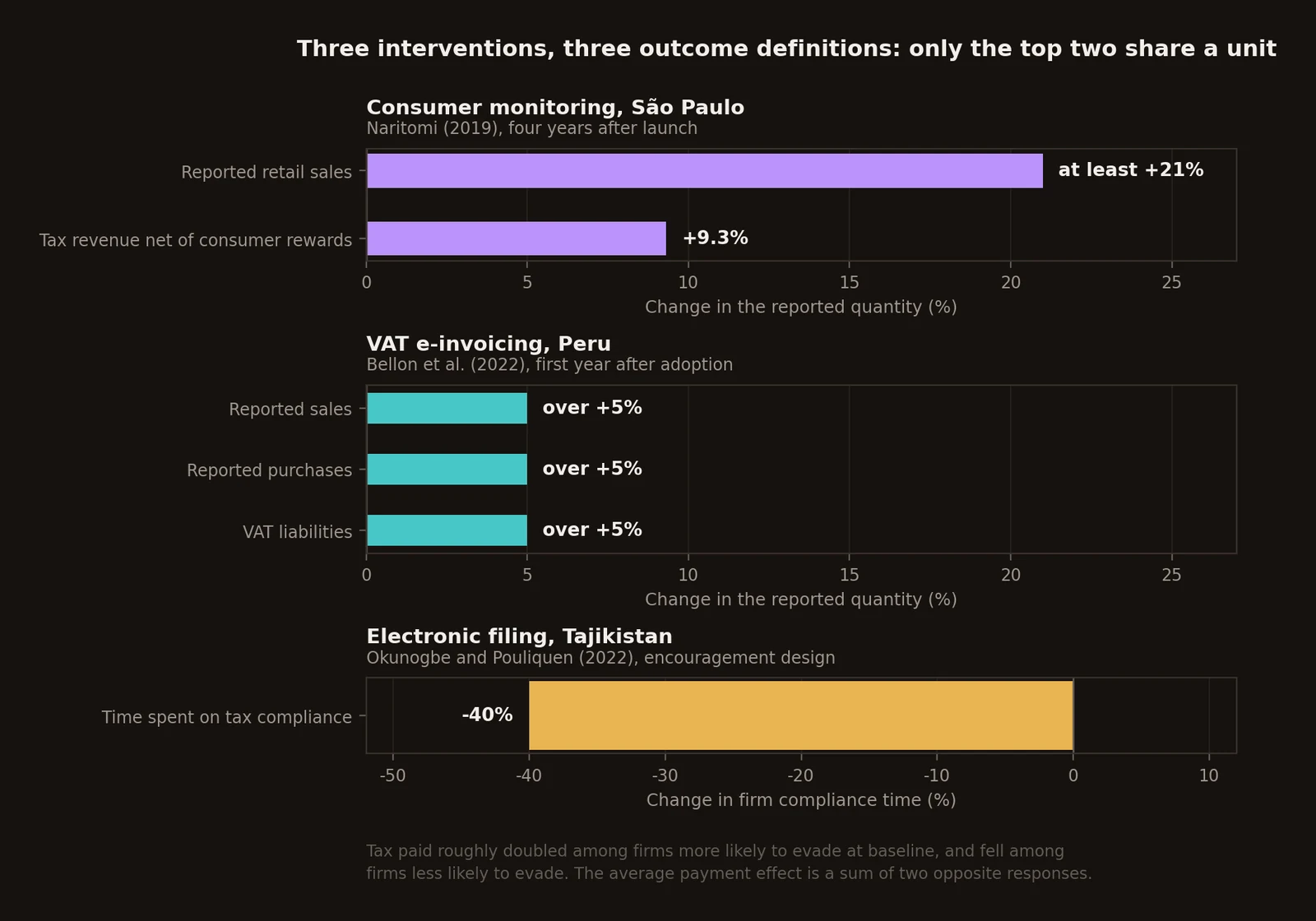
Naritomi extends that logic to the last link, final-consumer transactions, where ordinary VAT self-enforcement is weakest because the buyer needs no invoice for a credit. A consumer-reward and whistle-blowing scheme in São Paulo raised reported retail sales by at least 21 per cent over four years, with tax revenue net of the rewards up 9.3 per cent. Four years is unusually informative in a literature where most communication experiments are measured over weeks.

Information is not sufficient when another margin is available. Carrillo, Pomeranz and Singhal studied Ecuadorian firms notified of revenue discrepancies found through third-party data. Many did nothing. Those that raised reported revenue offset almost all of it by raising reported costs: 96 cents of extra cost per dollar of revenue adjustment, leaving very little extra tax. Verifying sales while leaving deductions unverified moves misreporting rather than removing it.

Intrinsic motivation is real and its external validity should not be oversold. Dwenger and co-authors studied a German local church tax that had historically operated with effectively zero deterrence for some taxpayers, and still observed substantial compliance. That is unusually clean evidence that not all payment is bought with expected punishment. Kirchler, Hoelzl and Wahl's slippery-slope framework rationalises the distinction as enforced compliance flowing from power and voluntary compliance from trust. These establish that non-deterrence motives exist. They do not establish that a one-unit increase in national institutional trust has a transportable causal effect on tax receipts anywhere.

That is worth stating plainly, because it is where the literature is weakest. Cross-country correlations between trust and tax morale are real, and reverse causality is immediate: predictable, effective tax institutions create trust, and trusted institutions may raise compliance. Survey response styles and cultural interpretation of the same question add another layer. Country fixed effects absorb stable traits; they cannot manufacture exogenous variation in trust.

What field interventions move, in the units they were measured in

The cleanest quantitative summary for behavioural messages is Antinyan and Asatryan's 2025 meta-analysis. Simple reminders raise extensive-margin compliance by 2.7 percentage points. Content referring to tax morale adds about 1.4 points on top of the reminder; deterrence content adds 3.2. In the subset that reports control means, roughly a quarter of control taxpayers were compliant, so these are increments on a low base among a heavily selected population, much of it already delinquent.

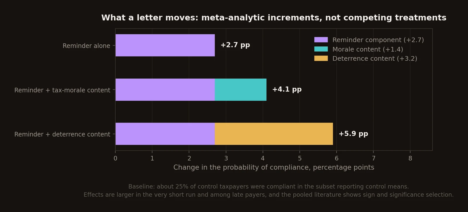
Drawing those three numbers as free-standing dots, which is the obvious chart and the one the research draft specified, says something false: it implies three competing interventions of which deterrence is the largest. Two of the three are increments on top of the reminder, so they belong in a stack. The distinction is not cosmetic, because an administration choosing between letters is choosing what to put in the letter, not whether to send one.

Those headline effects carry an unusually strong caveat. The broadest publication-bias sample contains 928 estimates from 65 papers, and the funnel and regression diagnostics indicate selection towards positive signs and statistical significance, with patterns consistent with selective reporting around conventional thresholds. Random assignment protects the internal validity of one experiment. It does nothing to protect the published literature from selective choice of outcomes, specifications, treatment arms or papers. The 2.7, 1.4 and 3.2 are descriptive summaries of the available experimental record, not structural constants.

Deterrence messages also need separating from deterrence. A letter mentioning audits changes salience and beliefs about enforcement; it need not change the objective audit probability at all. Bergolo and co-authors randomised messages to 20,440 small and medium firms paying more than 200 million dollars in tax a year, and found that audit-related information changes compliance in ways the canonical expected-utility model does not fully capture. Unless an experiment randomises actual audit probability, a treatment arm labelled "audit threat" is an intervention in perceived enforcement.

Digitalisation works through a different channel again. Bellon and co-authors' phased VAT e-invoicing reform in Peru raised reported sales, purchases and VAT liabilities by over 5 per cent in the first year after adoption, with larger effects among smaller firms and in sectors thought to have higher baseline non-compliance, and with spillovers through trading partners consistent with an information-network mechanism rather than convenience.

Electronic filing changes transaction costs and the taxpayer-official interface. Okunogbe and Pouliquen's encouragement design in Tajikistan cut the time firms spent on tax compliance by about 40 per cent. The payment effects are the interesting part: tax paid roughly doubled among firms more likely to evade at baseline, and fell among firms less likely to evade. An average effect that pools two opposite responses is not a summary of anything. The likely mechanism is that removing the face-to-face interface disrupts informal bargaining in both directions, which is not what "simplification" means.

Prefilled returns are genuinely ambiguous. They cut clerical burden when third-party information is complete and correct, and they can anchor: a taxpayer may infer that anything absent from the prefill is either unimportant or already known to the administration. Kotakorpi and Laamanen's Finnish natural experiment found significant reductions in non-prefilled deductions and in self-reported income, with prefilled deductions rising and total taxable income and tax paid unchanged. Administrative convenience and reporting accuracy are not the same objective.

Cooperative-compliance programmes are the clearest case of institutional adoption running ahead of causal measurement. OECD frameworks describe programmes built on transparency, tax-control frameworks and greater certainty for large business, and observational work finds associations between participation, tax-risk management and perceived certainty. The sources verified for this article do not contain a transportable randomised or quasi-experimental estimate of the effect on correctly reported tax. The right entry is "not credibly identified", not a qualitative claim converted into a number.

Intervention	Population and outcome	Effect size that can actually be stated	Qualification
Simple reminder	Extensive-margin filing and payment across the RCT literature	+2.7 percentage points	Larger in the very short run; publication selection detected
Tax-morale message	RCT literature, incremental to a reminder	+1.4 percentage points	Heterogeneous, generally weaker than deterrence content
Deterrence message	RCT literature, incremental to a reminder	+3.2 percentage points	Measures enforcement salience, not audit probability
Consumer-generated third-party information	Retail firms, reported sales and net revenue	Sales at least +21% over four years; revenue net of rewards +9.3%	Persistent over four years in the studied setting
VAT e-invoicing	Firms under a phased mandate	Sales, purchases and VAT liabilities over +5% in year one	Stronger among smaller and higher-risk firms; network spillovers matter
Electronic filing	Firms encouraged experimentally into e-filing	Compliance time -40%; tax paid roughly doubled in the high-baseline-evasion subgroup and fell in the low one	The average is a sum of opposite responses and should not be quoted alone
Detected-discrepancy notification	Firms with third-party revenue mismatches	Responders raised reported costs 96 cents per dollar of revenue adjustment	Offsetting-margin response; tax collected rose only modestly
Actual audit	Random-audit experiments and subsequent reporting	Direction and margin credibly identified; no globally comparable magnitude	Depends almost entirely on self-reported versus third-party-reported income
Prefilled returns	Natural experiment in partial prefiling	No verified universal positive effect; some non-prefilled items fell	Possible anchoring channel; total tax paid unchanged
Cooperative compliance	Large-business programmes	No causal effect size verified	Evidence is institutional and observational

The combined evidence rejects a one-dimensional theory. Third-party information and withholding make evasion difficult; actual or perceived enforcement changes expected costs; reminders address limited attention; electronic systems cut errors and face-to-face transaction costs; intrinsic motives sustain some compliance under weak deterrence. The empirical strength of those five statements is very unequal. Information-reporting mechanisms and randomised communications are unusually well identified. National trust-causes-compliance regressions and cooperative-compliance narratives are not.

Four questions, four models

The same administrative dataset supports at least four different questions. What is the true level of compliance? What causes a change in it? Which cases are likely to be non-compliant? What will the aggregate indicator be next year? Measurement models, causal designs, risk scores and forecasts answer those in order, and substituting one output for another is the most common methodological error in this field, well ahead of choosing the wrong algorithm.

Cross-country determinants

The common specification is

with $y_{ct}$ a compliance or morale measure for country $c$ in year $t$, $\alpha_c$ country effects and $\lambda_t$ year effects. The estimand is a within-country conditional association between changes in $x$ and changes in $y$, net of common year shocks. Country fixed effects remove time-invariant differences. They do not solve simultaneity: institutional trust, administrative capacity, digitalisation and compliance all evolve together. They do not correct measurement error in a tax-gap dependent variable, and they do not fix non-invariance in a survey-based morale index. ISORA's own comparative documentation warns that changing administrative circumstances complicate even ten-year comparisons.

There is also a specification-search problem that rarely reaches the results section. Test trust, corruption, digital adoption, audit rates, tax rates, filing costs, income, inequality, informality and several lags of each without a pre-specified estimand, and filtering on $p < 0.05$ will manufacture a set of determinants that does not survive the next vintage of the dependent variable. Regularisation, hierarchical priors, false-discovery control and an explicit separation of exploratory from confirmatory analysis are the minimum. Absent an instrument, a discontinuity, a treatment assignment or another credible source of exogenous variation, the regression is descriptive, and that word belongs in the abstract rather than in a footnote.

Hierarchical Bayes, and what partial pooling is for

For taxpayer $i$ in segment $s$ of country $c$,

with

The subscript on $\gamma_{sc}$ is doing real work and is easy to lose. It says the segment effect is nested within country: micro-enterprises in one jurisdiction need not behave like micro-enterprises in another. A model that gives the segment effect five parameters shared across every jurisdiction is a different and much stronger assumption, and the notation and the code have to agree about which one is being fitted. They frequently do not.

The estimand is a posterior distribution over individual or segment compliance probability, together with population-level effects. Partial pooling shrinks noisy small-cell estimates towards the wider distribution, which matters enormously when one jurisdiction contributes hundreds of observations and another contributes thousands. Shrinkage is not a licence to pool incomparable things: the likelihood still has to refer to an outcome defined the same way across every unit, and no amount of hierarchy repairs a filing-rate denominator that means different things in different countries.

The code below runs against a simulated panel whose truth is known, which is the only way to check that the machinery is doing what it claims. The data-generating process: 12 countries and 5 segments, country intercepts drawn $\mathcal{N}(0, 0.55^2)$, segment-within-country deviations $\mathcal{N}(0, 0.35^2)$, three standardised covariates with coefficients $(0.85, -0.40, 0.20)$, a global intercept of $0.60$, and country sample sizes drawn from 45 to 900 so the panel is as unbalanced as a real one.

import arviz as az
import numpy as np
import pandas as pd
import pymc as pm

df = pd.read_csv("compliance_microdata.csv")

required = {"compliant", "country", "segment", "x1", "x2", "x3"}
missing = required.difference(df.columns)
if missing:
    raise ValueError(f"Missing columns: {sorted(missing)}")
if not set(df["compliant"].dropna().unique()).issubset({0, 1}):
    raise ValueError("'compliant' must be binary.")
df = df.dropna(subset=list(required)).copy()

country_codes, countries = pd.factorize(df["country"], sort=True)
segment_codes, segments = pd.factorize(df["segment"], sort=True)

X_cols = ["x1", "x2", "x3"]
X = df[X_cols].to_numpy(dtype=float)
scale = X.std(axis=0, ddof=0)
scale[scale == 0] = 1.0          # a constant column is useless, not fatal
X = (X - X.mean(axis=0)) / scale

coords = {
    "obs": np.arange(len(df)),
    "country": countries.tolist(),
    "segment": segments.tolist(),
    "feature": X_cols,
}

with pm.Model(coords=coords) as model:
    country_idx = pm.Data("country_idx", country_codes, dims="obs")
    segment_idx = pm.Data("segment_idx", segment_codes, dims="obs")
    X_data = pm.Data("X", X, dims=("obs", "feature"))

    intercept = pm.Normal("intercept", mu=0.0, sigma=1.5)

    # Non-centred throughout. The centred form couples each group mean to its
    # own scale and produces the funnel geometry that shows up as divergences
    # long before it shows up as a wrong answer.
    sigma_country = pm.HalfNormal("sigma_country", sigma=1.0)
    z_country = pm.Normal("z_country", 0.0, 1.0, dims="country")
    country_effect = pm.Deterministic(
        "country_effect", z_country * sigma_country, dims="country"
    )

    # Nested, matching gamma_{sc}: one deviation per country-segment cell,
    # not five shared across the world.
    sigma_segment = pm.HalfNormal("sigma_segment", sigma=1.0)
    z_segment = pm.Normal("z_segment", 0.0, 1.0, dims=("country", "segment"))
    segment_effect = pm.Deterministic(
        "segment_effect", z_segment * sigma_segment, dims=("country", "segment")
    )

    beta = pm.Normal("beta", mu=0.0, sigma=1.0, dims="feature")

    eta = (
        intercept
        + country_effect[country_idx]
        + segment_effect[country_idx, segment_idx]
        + pm.math.dot(X_data, beta)
    )

    pm.Bernoulli("compliant", logit_p=eta,
                 observed=df["compliant"].to_numpy(), dims="obs")

    idata = pm.sample(draws=1_000, tune=1_000, chains=4, cores=4,
                      target_accept=0.90, random_seed=20260830)

    # extend_inferencedata, not a bare call: sample_posterior_predictive on its
    # own returns an InferenceData carrying only a posterior_predictive group,
    # and az.plot_ppc needs observed_data as well. Without this the check that
    # is supposed to catch a bad model is itself the thing that breaks.
    pm.sample_posterior_predictive(
        idata, var_names=["compliant"], random_seed=20260830,
        extend_inferencedata=True,
    )

print(az.summary(
    idata,
    var_names=["intercept", "sigma_country", "sigma_segment", "beta"],
    round_to=3,
))
print("Divergences:", int(idata.sample_stats["diverging"].sum()))

                mean     sd  hdi_3%  hdi_97%  mcse_mean  mcse_sd  ess_bulk  ess_tail  r_hat
intercept      0.662  0.204   0.254    1.041      0.006    0.004  1265.420  1736.140  1.003
sigma_country  0.645  0.201   0.312    1.016      0.006    0.005  1231.296  1636.690  1.001
sigma_segment  0.441  0.073   0.316    0.584      0.002    0.001  1389.388  2425.155  1.001
beta[x1]       0.831  0.040   0.760    0.907      0.001    0.001  6232.936  2920.554  1.001
beta[x2]      -0.399  0.036  -0.463   -0.330      0.000    0.001  6945.731  2792.861  1.003
beta[x3]       0.164  0.034   0.100    0.227      0.000    0.001  6860.902  2595.898  0.999

Divergences: 0

Posterior predictive: observed country filing rate inside the 95% replicated interval for 12 of 12 countries
Mean absolute shrinkage: 0.057 in the smaller half of cells, 0.028 in the larger half

The model recovers what generated the data: 0.831 against a true 0.85, -0.399 against -0.40, 0.164 against 0.20, and group scales of 0.645 and 0.441 against 0.55 and 0.35. R-hat is at most 1.003, effective sample sizes run from 1,200 to 6,900, there are no divergences, and the observed filing rate falls inside the 95% replicated interval for all twelve countries. That is what a model that is working looks like, and it is the baseline against which the meta-analysis section's failure is worth reading. Getting there needs the diagnostics read before the coefficients: R-hat, effective sample size and the divergence count are preconditions for looking at a posterior at all, rank-normalised split-R-hat and ESS are the current recommendation, and a plausible-looking posterior mean from a chain that never explored the space is not evidence of anything. Running those chains at a size where that check is expensive, and streaming the convergence metrics somewhere a human can watch them arrive, is the subject of a separate note on distributed MCMC pipelines.

One practical note, because it is the difference between this block running and not. pytensor compiles the model graph to C, and where no C compiler is installed it falls back to evaluating the graph in Python without saying so loudly. Measured on this model, one gradient takes 119 ms that way against 0.106 ms through numba, a factor of 1,120; NUTS needs tens of gradients per draw, so the fallback turns a 36-second run into several hours per chain. compile_kwargs={"mode": "NUMBA"} needs no compiler and is worth setting by default on any machine where the C toolchain is not certain.

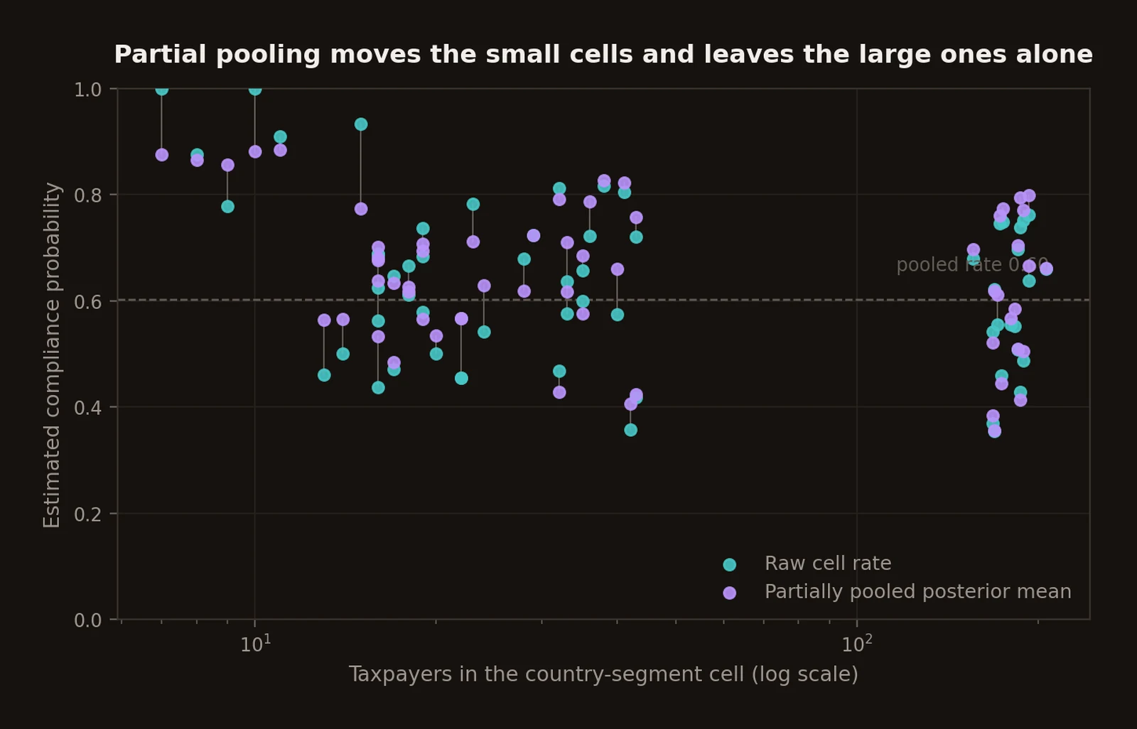
The figure is the argument for the model. It holds 60 country-segment cells ranging from 7 taxpayers to 206, and the raw rates behave as sample size dictates rather than as behaviour does: among the smallest quarter of cells the raw rate runs from 0.44 all the way to 1.00, two cells apparently achieving perfect compliance on the strength of six and ten observations, while among the largest quarter it stays inside 0.43 to 0.76. Partial pooling moves the small cells and leaves the large ones where they are: mean absolute movement is 0.057 in the smaller half of cells against 0.028 in the larger half.

That is not the model overriding the data. It is the model declining to believe a rate of 1.00 that six draws can produce by accident, while barely touching a rate estimated on two hundred. An administration that ranks jurisdictions or segments on raw rates is ranking them substantially on how many taxpayers each one happens to contain.

Meta-analysis, and the selection that comes with a published literature

For an independent effect estimate $\widehat\theta_j$ with standard error $s_j$,

where $\mu$ is the pooled mean and $\tau$ the between-study heterogeneity. Before any of that, outcomes have to be mapped onto one estimand, preferably the percentage-point change in an extensive-margin event such as filing or paying by a deadline. Percentage changes in revenue, log declared income and percentage-point payment responses cannot be pooled without an explicit effect-size transformation, and multiple arms from one experiment are correlated, so treating them as independent understates uncertainty.

Heterogeneity is the finding, not the nuisance. A large $\tau$ means "the average nudge effect" has limited predictive content for the next administration, which is what the reader actually wants to know. The quantity to report is therefore the prediction interval for a new study, not only the credible interval for the mean.

Publication-bias diagnostics each answer a different question. Funnel asymmetry asks whether less precise estimates are systematically larger. Egger's regression formalises that as a standard normal deviate regressed on precision, where the intercept is the test. PET and PEESE regress the effect on the standard error and on the sampling variance respectively, under stronger functional assumptions, and read the intercept as the effect at infinite precision. A p-curve inspects the distribution of significant results and can reveal concentration just under a threshold. None of them corrects publication bias; together they produce a sensitivity envelope.

Running them on a real literature tells you the envelope but never whether it is right, because the truth is unobserved. So the code below runs on a synthetic literature whose selection rule is known: 140 candidate studies, a true mean effect of 1.20 percentage points, between-study heterogeneity of 0.90, and a filter that publishes a study with certainty when $p < 0.05$ and with probability 0.20 otherwise. Sixty-eight of the 140 survive. The mean effect among all 140 candidates is 1.086; among the 68 published it is 1.838.

import arviz as az
import numpy as np
import pandas as pd
import pymc as pm
import statsmodels.api as sm
from scipy.stats import norm

df = pd.read_csv("meta_effects.csv")
required = {"effect_pp", "se_pp"}
missing = required.difference(df.columns)
if missing:
    raise ValueError(f"Missing columns: {sorted(missing)}")

df = df.replace([np.inf, -np.inf], np.nan).dropna(subset=list(required))
if (df["se_pp"] <= 0).any():
    raise ValueError("All standard errors must be positive.")

y = df["effect_pp"].to_numpy(float)
se = df["se_pp"].to_numpy(float)
J = len(df)

with pm.Model() as meta_model:
    mu = pm.Normal("mu", mu=0.0, sigma=10.0)
    tau = pm.HalfNormal("tau", sigma=5.0)
    theta = pm.Normal("theta", mu=mu, sigma=tau, shape=J)
    pm.Normal("effect", mu=theta, sigma=se, observed=y)

    idata = pm.sample(draws=3_000, tune=3_000, chains=4, cores=4,
                      target_accept=0.95, random_seed=20260830)

print(az.summary(idata, var_names=["mu", "tau"], round_to=3))

# The question an administration asks is what the NEXT trial will do, so the
# interval that matters is predictive, not the credible interval for the mean.
draws_mu = idata.posterior["mu"].values.ravel()
draws_tau = idata.posterior["tau"].values.ravel()
predictive = np.random.default_rng(20260830).normal(draws_mu, draws_tau)

precision = 1.0 / se
snd = y / se

# Egger: standard normal deviate on precision. The intercept is the test.
egger = sm.OLS(snd, sm.add_constant(precision)).fit(cov_type="HC3")
# PET: effect on standard error, inverse-variance weighted.
pet = sm.WLS(y, sm.add_constant(se), weights=1.0 / se ** 2).fit(cov_type="HC3")
# PEESE: effect on sampling variance, same weights.
peese = sm.WLS(y, sm.add_constant(se ** 2), weights=1.0 / se ** 2).fit(cov_type="HC3")

p_two_sided = 2.0 * norm.sf(np.abs(y / se))
p_sig = p_two_sided[p_two_sided < 0.05]

      mean     sd  hdi_3%  hdi_97%  mcse_mean  mcse_sd  ess_bulk  ess_tail  r_hat
mu   1.696  0.126   1.464    1.941      0.001    0.001  8799.684  9526.840    1.0
tau  0.735  0.103   0.544    0.922      0.001    0.001  5075.282  7865.185    1.0

Divergences: 0
Pooled mean            1.696 pp [1.449, 1.945]
Prediction interval    [0.220, 3.202] pp for the next study
True mean in the DGP   1.200 pp

Egger intercept        +1.446 (SE 0.897, p = 0.1071)   non-zero means small studies report larger effects
PET intercept          +0.744 (SE 0.671, p = 0.2672)   effect extrapolated to SE = 0
PEESE intercept        +1.189 (SE 0.392, p = 0.0024)

Published estimates    68
Significant at 5%      55 (80.9%)
Naive published mean   1.838 pp   (+53% against the truth)

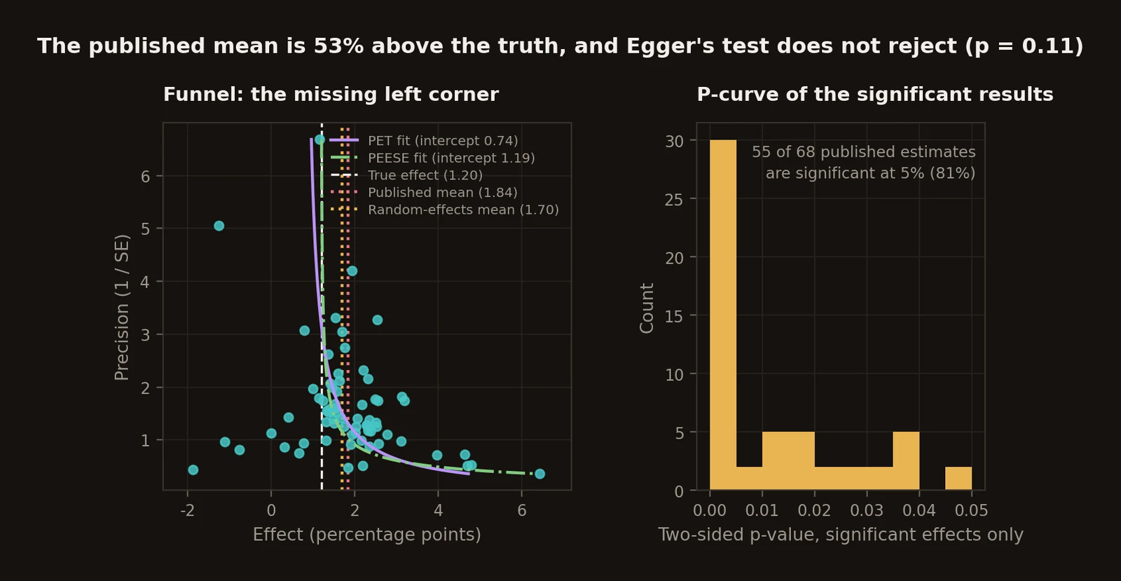
The point of running this on known data is that every number can be checked, and three of them are not what a reader would expect.

The naive published mean, 1.838, overstates the truth by 53 per cent. The Bayesian random-effects model does not rescue it. Pooling correctly with respect to sampling error and heterogeneity, but not with respect to selection, gives a posterior mean of 1.696 with a 95% credible interval of [1.449, 1.945], which excludes the true 1.20 outright. Every convergence diagnostic is clean: R-hat 1.0, effective sample sizes in the thousands, no divergences. A well-specified hierarchical model fitted to a filtered sample is a precise, well-behaved estimate of the filtered sample.

Egger's test then fails. The intercept is +1.446 with a standard error of 0.897 and p = 0.107, so on a literature built with a selection rule that is known because it was written into the generator, the standard funnel-asymmetry test does not reject at five per cent. Sixty-eight studies is not many and funnel-based tests are badly underpowered at that size. A non-significant Egger test is not evidence that selection is absent, and a paper that reports one as reassurance is reporting the absence of power.

PET and PEESE then disagree with each other. PET, which extrapolates the effect to zero standard error, returns +0.744 with p = 0.267 and undershoots. PEESE, which regresses on the sampling variance instead, returns +1.189, which is 0.011 away from the true 1.200. The conventional PET-PEESE decision rule is to run PET first and only move to PEESE if PET's intercept is significantly positive. Here PET is not significant, so the rule stops there and concludes there is no effect to correct, discarding the one estimator that got the answer right. Two estimators that differ this much on the same data are telling you that the functional form is carrying the estimate, not the evidence.

What does fire is the crudest diagnostic available. Fifty-five of the 68 published estimates, 81 per cent, are significant at five per cent. With between-study heterogeneity of 0.9 and these standard errors, an unfiltered literature does not produce that share, and no test is needed to see it. The p-curve is right-skewed, so a real effect exists underneath. The significance share says the record has been filtered on the way to publication.

Read Antinyan and Asatryan's own diagnostics on the real literature in that light. They do not show that reminders do nothing; their p-curve evidence points the same way as the one above. They show that the published record carries selection by sign and significance, which makes 2.7 percentage points a description of what has been published rather than an unbiased estimate of what a letter does. The wrong response is to invent a correction factor and multiply. The right one is to report the pooled mean, the prediction interval and the full set of bias diagnostics together, to say plainly which of them had the power to detect anything, and to let the width of that envelope be the answer.

Causal identification in administrative settings

A randomised communication trial estimates an intention-to-treat effect,

if assignment is random, attrition and outcome measurement do not depend differentially on assignment, and spillovers are either absent or part of the intended estimand. The main interpretive danger here is treatment ambiguity rather than assignment: an audit letter estimates the effect of telling taxpayers about enforcement, which is not the effect of enforcement.

Administrative reforms usually cannot be randomised at the individual level. Difference-in-differences compares treated and untreated units around a reform, and the identifying assumption is about untreated potential-outcome trends, not about observed pre-trends looking parallel. With staggered adoption and heterogeneous effects, a conventional two-way fixed-effects event study forms contaminated comparisons between already-treated and newly-treated groups; group-time estimators and interaction-weighted event studies avoid that specific failure but still need a defensible comparison group and no anticipation. Synthetic control suits a single large reform when a weighted donor pool reproduces the treated unit's pre-reform path. Bunching and regression discontinuity exploit registration or turnover thresholds, but only where the counterfactual density or the potential outcomes would have been smooth and no other rule changes at the same point.

That last condition is the one that fails quietly. Almunia and López-Rodríguez's work on size-dependent monitoring in Spain shows why thresholds are informative: firms bunch below the large-taxpayer eligibility line, and the excess mass is a response to the regime. It is a response to the entire bundle at that line. If registration requirements, reporting frequency, audit intensity and liability all change at the same revenue figure, no amount of bandwidth tuning will separate them without additional structure.

Predictive risk modelling

Prediction begins with a label, and the label is an administrative choice rather than a fact. "Non-compliant" can mean late filing, debt unpaid after 30 days, any audit adjustment, an adjustment above a materiality threshold, confirmed fraud, or expected recoverable revenue. Those are different prediction problems with different populations.

Training on "audit adjustment greater than zero" also creates selective-label bias, because operational audits are targeted. The model then learns the distribution of non-compliance among audited taxpayers, which is the population the previous selection rule chose, and its errors are invisible for everybody else. Random measurement programmes such as the IRS National Research Program and HMRC's random enquiries are usually justified as statistical reporting; their more valuable property is that they provide a less selected frame to train and validate on.

Discrimination and calibration are separate properties and get confused constantly. ROC-AUC asks whether higher-risk cases tend to outrank lower-risk ones. Calibration asks whether a predicted 0.20 corresponds to an event frequency near 20 per cent among comparable cases. A model can rank well and calibrate badly, and for allocating a fixed review capacity the operationally meaningful quantity is top-decile lift:

where $D_{1}$ is the top decile of the ranking. Note "of the ranking". Taking the top decile as everything above the 90th percentile of predicted probability is not the same set when a tree ensemble produces ties, and the two definitions can differ by several percentage points of coverage. Brier score measures squared probabilistic error and so responds to calibration as well as to ranking.

Feature attribution needs the same care. Impurity-based importance from a tree ensemble rewards variables with many possible split points and distributes credit unpredictably among correlated variables. Permutation importance asks a more operational question, how much held-out performance degrades when a feature's association with the outcome is broken, and is still not causal importance: correlated substitutes mask one another, so a feature can look unimportant precisely because the model can reconstruct it.

The code below runs on a simulated filing panel with a regime change built into the test period: 24 monthly periods, 900 taxpayers each, and from period 19 the coefficient on the third-party mismatch feature halves, standing in for an e-invoicing mandate that removes part of the opportunity. The model is therefore trained in one regime and scored in another, which is the situation every production score is in and almost no evaluation reproduces.

import numpy as np
import pandas as pd
from sklearn.calibration import CalibratedClassifierCV, calibration_curve
from sklearn.compose import ColumnTransformer
from sklearn.ensemble import RandomForestClassifier
from sklearn.impute import SimpleImputer
from sklearn.inspection import permutation_importance
from sklearn.metrics import (average_precision_score, brier_score_loss,
                             roc_auc_score)
from sklearn.model_selection import TimeSeriesSplit
from sklearn.pipeline import Pipeline
from sklearn.preprocessing import OneHotEncoder

df = pd.read_csv("risk_scoring.csv", parse_dates=["filing_period"])
if "outcome" not in df or "filing_period" not in df:
    raise ValueError("Input requires 'outcome' and 'filing_period'.")

df = df.sort_values("filing_period").dropna(subset=["outcome"]).copy()
if not set(df["outcome"].unique()).issubset({0, 1}):
    raise ValueError("'outcome' must be binary.")

cutoff = df["filing_period"].quantile(0.80)
train = df[df["filing_period"] <= cutoff].copy()
test = df[df["filing_period"] > cutoff].copy()

features = [c for c in df.columns if c not in {"outcome", "filing_period"}]
X_train, y_train = train[features], train["outcome"]
X_test, y_test = test[features], test["outcome"]

numeric = X_train.select_dtypes(include=np.number).columns.tolist()
categorical = [c for c in features if c not in numeric]

preprocess = ColumnTransformer(transformers=[
    ("num", Pipeline([("impute", SimpleImputer(strategy="median"))]), numeric),
    ("cat", Pipeline([
        ("impute", SimpleImputer(strategy="most_frequent")),
        ("onehot", OneHotEncoder(handle_unknown="ignore")),
    ]), categorical),
])

# No class_weight. Reweighting shifts every predicted probability away from the
# base rate, which is exactly the quantity the calibration step then has to
# undo; it does not change the ranking, and it makes calibration harder. A
# score meant to be read as a probability should not carry both.
base = Pipeline([
    ("prep", preprocess),
    ("model", RandomForestClassifier(n_estimators=800, min_samples_leaf=20,
                                     random_state=20260830, n_jobs=-1)),
])

# TimeSeriesSplit, not cv=5. Random folds in a design whose whole point is a
# temporal holdout let a taxpayer's later periods calibrate the score applied
# to their earlier ones.
model = CalibratedClassifierCV(estimator=base, method="isotonic",
                               cv=TimeSeriesSplit(n_splits=5))
model.fit(X_train, y_train)

p = model.predict_proba(X_test)[:, 1]
roc = roc_auc_score(y_test, p)
pr_auc = average_precision_score(y_test, p)
brier = brier_score_loss(y_test, p)

# Lift is a property of the RANKING, so the top decile is the top 10% of cases,
# not everything above a fixed probability. With ties in a tree ensemble the
# two are different sets.
order = np.argsort(-p, kind="stable")
k = max(1, int(round(0.10 * len(p))))
top = np.zeros(len(p), dtype=bool)
top[order[:k]] = True

base_rate = float(y_test.mean())
lift_10 = float(y_test.to_numpy()[top].mean()) / base_rate

frac_pos, mean_pred = calibration_curve(y_test, p, n_bins=10, strategy="quantile")

perm = permutation_importance(model, X_test, y_test, scoring="neg_brier_score",
                              n_repeats=20, random_state=20260830, n_jobs=-1)
importance = (
    pd.DataFrame({"feature": features,
                  "importance_mean": perm.importances_mean,
                  "importance_sd": perm.importances_std})
    .sort_values("importance_mean", ascending=False)
)

Train 2024-01-01 to 2025-08-01, 18,000 rows
Test  2025-09-01 to 2025-12-01, 3,600 rows

roc_auc          0.6832
pr_auc           0.3197
brier            0.1475   (base-rate-only model: 0.1501)
base rate        0.1839
top-decile rate  0.3750
top_decile_lift  2.0393
worst calibration bin deviates by 0.1859

             feature  importance_mean  importance_sd
              sector          0.00795        0.00122
third_party_mismatch          0.00784        0.00090
       arrears_count          0.00525        0.00071
   prior_late_filing          0.00455        0.00069
   months_registered          0.00396        0.00045
          amendments          0.00098        0.00023
        turnover_log          0.00033        0.00021

Predicted against observed positive rate, by test period:
                   n  observed  predicted
filing_period
2025-09-01     900.0    0.1778     0.2530
2025-10-01     900.0    0.1867     0.2525
2025-11-01     900.0    0.1944     0.2526
2025-12-01     900.0    0.1767     0.2505

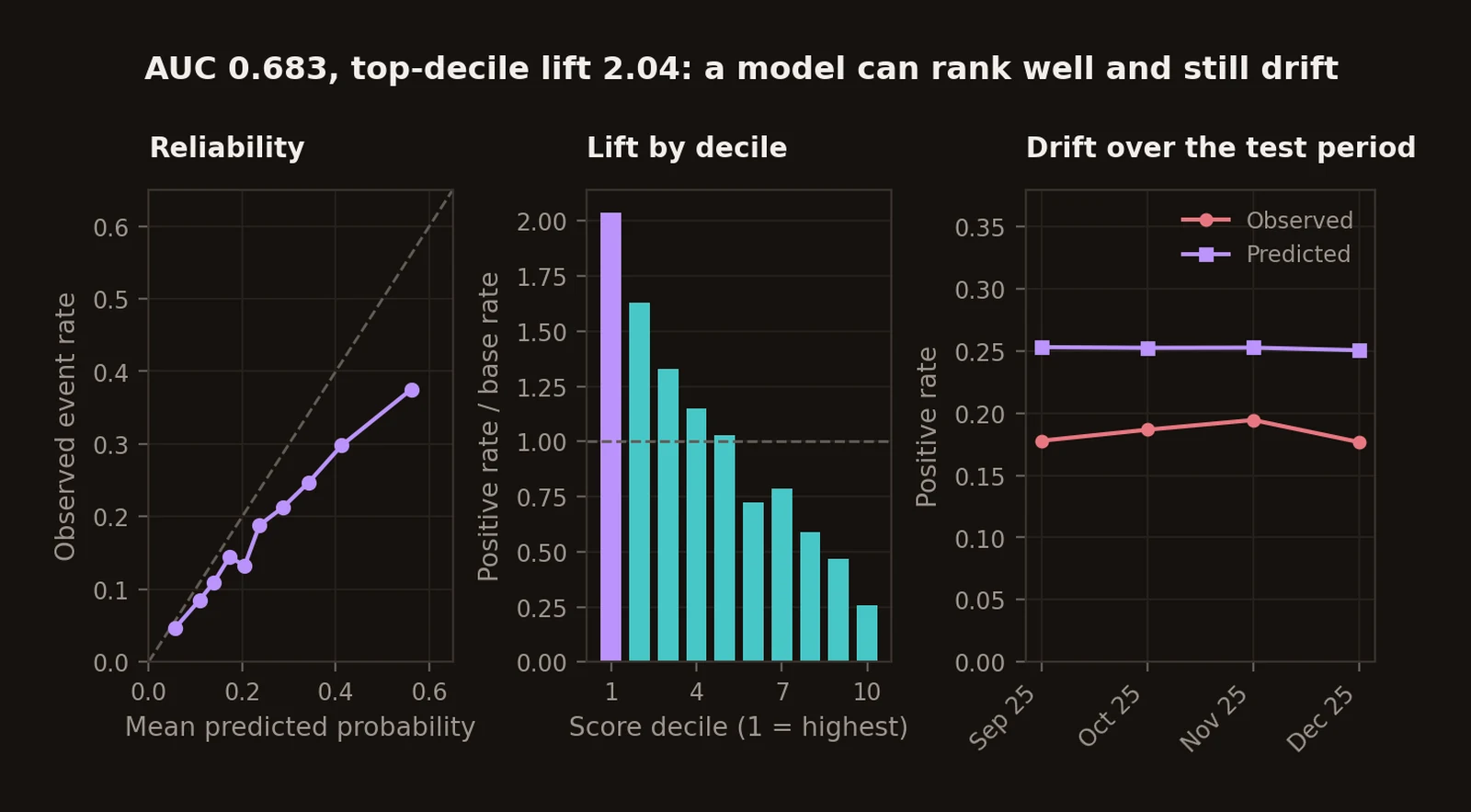
Read those numbers together and they say one thing. The ranking works: the top decile carries 2.04 times the base rate and the decile lift falls monotonically from 2.04 to 0.25, which is exactly what an audit queue needs. The probabilities do not: the model predicts about 0.25 in every test month against an observed 0.18, the reliability curve sits below the diagonal along its whole length, and the worst bin is out by 0.19. The Brier score, 0.1475, barely beats the 0.1501 a model that only ever predicts the base rate would score. Ranking value survived the regime change; probabilistic value very nearly did not. That is the whole reason to report both, and the reason the trigger for re-estimation should be the calibration gap rather than the AUC, which will look fine for a long time after the probabilities stop meaning anything.

Class imbalance does not justify oversampling before a temporal split or a calibration step. What matters is whether the final score is validated on a population that resembles the decision population, and here it was not: the training period ran at a 25 per cent positive rate and the test period at 18, because the simulated e-invoicing mandate removed part of the opportunity the model had learned to detect. Drift monitoring therefore needs feature-distribution checks, outcome-rate checks, rolling calibration and periodic re-estimation.

Fairness changes character when a score can trigger coercive action. A purely revenue-maximising ranking will repeatedly expose the groups with richer observable data to audit and leave the hard-to-observe under-sampled, and that feedback then changes the labels available to the next model. A defensible production system needs logged model versions, immutable feature snapshots, documented exclusion rules, subgroup error analysis, human review before consequential action, and a route by which factual errors in administrative data can be corrected. OECD's recent tax-administration work documents how widespread predictive analytics has become in this sector, which makes model governance infrastructure rather than theory.

Method	Estimand	Critical assumption	Characteristic failure	Minimum diagnostic
Top-down gap model	Macro potential liability minus observed revenue	National accounts and legal mapping approximate the true potential base	The residual mixes non-compliance with measurement and model error	Sensitivity to base, exemptions, timing and data revisions
Random-audit bottom-up model	Population under-reporting	Probability sampling and sufficiently accurate examination	Undetected evasion and non-filers sit outside the observed adjustment	Design weights, non-detection adjustment, uncertainty interval
Country-year fixed-effects panel	Within-country conditional association	No omitted time-varying confounder, for a causal reading	Trust, capacity and compliance are jointly determined	Specification stability, clustered uncertainty, multiplicity control
Hierarchical Bayes	Posterior group and individual probabilities	Exchangeability conditional on the hierarchy	Pooling incomparable groups; prior sensitivity	R-hat, ESS, divergences, posterior predictive checks
Random-effects meta-analysis	Distribution and mean of study effects	Comparable estimand, modelled dependence	Pseudoreplication, heterogeneity, publication selection	$\tau$, prediction interval, funnel, Egger, PET-PEESE, p-curve
RCT	ITT, or treatment-on-treated under more assumptions	Random assignment, valid outcome measurement, controlled interference	The treatment is salience rather than enforcement	Balance, attrition, pre-specified outcomes, spillover analysis
DiD and event study	Average effect for treated cohorts	Credible untreated counterfactual trends	Staggered-treatment contamination, anticipation	Event-time diagnostics, cohort-specific estimator
Synthetic control	Effect on one or few treated units	The donor pool reproduces the counterfactual	Poor pre-fit, or a concurrent idiosyncratic shock	Pre-fit RMSPE, placebo and permutation exercises
Bunching and RD	Local response at a threshold	Smooth counterfactual absent the threshold	Several rules change at the same point; manipulation	Density and bandwidth robustness
Risk classifier	Probability or ranking of an operational label	The label is meaningful and the training distribution transports	Selected labels, leakage, drift, miscalibration	Temporal holdout, Brier, reliability curve, lift, drift tests

Forecasting a series that is partly a forecast already

Forecasting compliance is harder than forecasting a mature macroeconomic series, and not because the behaviour is more volatile. It is because the published indicators are annual, short, revised, and partly model-generated. A tax-gap series can move because compliance moved, because the national accounts were revised, because an audit study supplied new information, or because the method changed. The IRS projections for 2021 and 2022 lean heavily on compliance behaviour estimated from completed audits of tax years 2014 to 2016, projected forward. The observed endpoint of a tax-gap series often already contains a substantial forecasting component, so a model fitted to it is in part forecasting somebody else's forecast.

A state-space representation makes the vintage problem explicit:

where $v$ indexes the data vintage, and the latent series evolves as

with $d_{c,t}$ a local trend, $\mathbf{z}$ contemporaneous macro or administrative covariates and $R$ marking known reforms. The additive vintage term $r_v$ is a modelling choice, not a fact about revisions: it says an edition shifts the whole series by a constant. The HMRC revisions above are not shaped like that, since 2022-23 moved by 1.8 points while 2024-25 is a first estimate, so a serious vintage model needs a component-specific or method-specific term instead. It is worth writing the simple version down anyway, because it makes visible that a regression on published values is implicitly assuming $r_v = 0$.

Two more things follow. Backtesting has to use rolling origins, and where possible each forecast should use the vintage that actually existed at the forecast date; scoring a 2019 forecast against a 2026-revised history leaks seven years of measurement improvement into the evaluation. And point error alone is not enough. A probabilistic forecast should be judged on interval coverage and a proper scoring rule such as the continuous ranked probability score, because a forecast that misses by two points with an honest wide interval is more useful than one that misses by 1.8 with an interval that is wrong about its own precision.

The code below runs on the real thing: HMRC's total tax gap as a percentage of theoretical liabilities, 2005-06 to 2024-25, twenty annual observations from the 2026 edition's online tables.

from math import pi, sqrt

import numpy as np
import pandas as pd
from scipy.stats import norm
from statsmodels.tsa.statespace.structural import UnobservedComponents

MIN_TRAIN, MAX_HORIZON = 10, 3


def normal_crps(observed, mean, sd):
    """CRPS for a Normal predictive distribution, in the units of the series."""
    sd = max(float(sd), 1e-12)
    z = (observed - mean) / sd
    return sd * (z * (2 * norm.cdf(z) - 1) + 2 * norm.pdf(z) - 1 / sqrt(pi))


def fit_and_forecast(train, horizon):
    # `level="local linear trend"` is a model *string*, and a model string
    # already fixes the irregular component. Passing `irregular=True` alongside
    # it does nothing except raise a SpecificationWarning.
    result = UnobservedComponents(train, level="local linear trend").fit(disp=False)
    pred = result.get_forecast(steps=horizon)

    mean = np.asarray(pred.predicted_mean)
    sf = pred.summary_frame(alpha=0.05)
    lower = sf[next(c for c in sf.columns if "lower" in c.lower())].to_numpy()
    upper = sf[next(c for c in sf.columns if "upper" in c.lower())].to_numpy()
    sd = (upper - lower) / (2 * norm.ppf(0.975))
    return mean, lower, upper, sd


series = gap_percentage_series("Total tax gap")     # HMRC online tables
y = series["gap_pct"].to_numpy(float)
labels = series["tax_year"].tolist()

records = []
for origin in range(MIN_TRAIN, len(y)):
    H = min(MAX_HORIZON, len(y) - origin)
    mean, lower, upper, sd = fit_and_forecast(y[:origin], H)
    for h in range(1, H + 1):
        actual = y[origin + h - 1]
        records.append({
            "origin": labels[origin - 1],
            "target": labels[origin + h - 1],
            "horizon": h,
            "actual": actual,
            "mean": mean[h - 1],
            "abs_error": abs(actual - mean[h - 1]),
            "covered_95": lower[h - 1] <= actual <= upper[h - 1],
            "crps": normal_crps(actual, mean[h - 1], sd[h - 1]),
        })

bt = pd.DataFrame(records)
report = bt.groupby("horizon").agg(
    mae=("abs_error", "mean"), crps=("crps", "mean"),
    coverage_95=("covered_95", "mean"), n_forecasts=("actual", "size"),
).round(3)

# A random walk is the honest yardstick for a short annual series: if the
# structural model cannot beat "next year looks like this year", the extra
# states are decoration.
naive = [{"horizon": h, "abs_error": abs(y[origin + h - 1] - y[origin - 1])}
         for origin in range(MIN_TRAIN, len(y))
         for h in range(1, min(MAX_HORIZON, len(y) - origin) + 1)]
naive_mae = pd.DataFrame(naive).groupby("horizon")["abs_error"].mean().round(3)

HMRC total tax gap, 2005-06 to 2024-25: 20 annual observations
Last two years (2023-24, 2024-25) are HMRC projections, not estimates

Rolling origins: 10, from 2014-15 to 2023-24
           mae   crps  coverage_95  n_forecasts
horizon
1        0.470  0.315        1.000           10
2        0.629  0.456        0.889            9
3        0.899  0.635        0.875            8

Random-walk benchmark MAE by horizon:
horizon
1    0.380
2    0.400
3    0.538

Three-step probabilistic forecast (percentage of theoretical liabilities):
tax_year  mean  lower_95  upper_95
 2025-26 6.347     5.366     7.328
 2026-27 6.360     5.050     7.670
 2027-28 6.373     4.748     7.999

The local linear trend loses to a random walk at every horizon, and by a widening margin: 0.470 against 0.380 one year out, 0.899 against 0.538 three years out. That result is worth more than a flattering one. Twenty annual observations, with a level and a slope to estimate and a variance for each, is not enough data to identify a trend, so the fitted slope tracks whichever direction the last few years happened to run and then extrapolates it into a series that turns. Look at the 2016-17 origin in the figure: five years of decline, a confidently continued decline, and an actual series that reversed the following year.

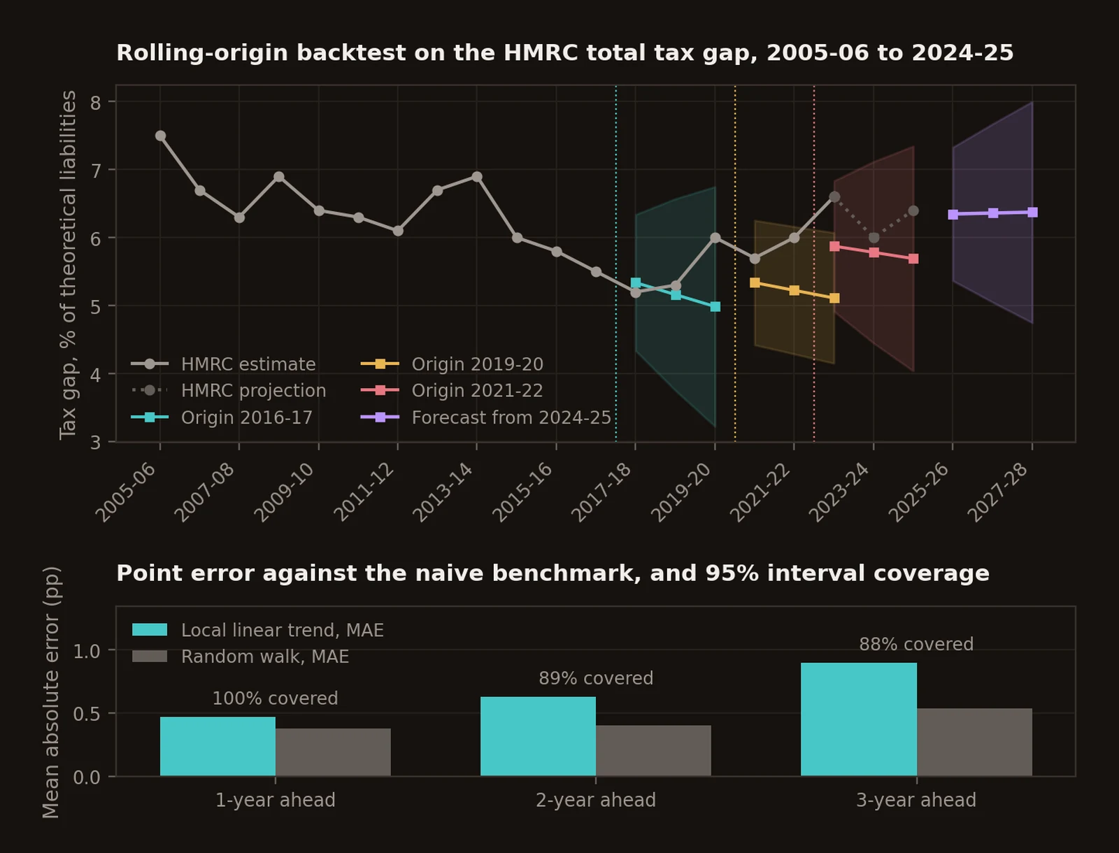
The intervals behave much better than the point forecasts: 100, 89 and 88 per cent coverage against a nominal 95, so the model is roughly honest about how little it knows even while its central path is worse than the naive one. That is the practical argument for scoring probabilistically. On mean absolute error the model is simply worse. On coverage it is usable, and an administration that needs a planning range rather than a number gets something defensible from it.

Which sets the horizon question honestly. One to three annual steps is a defensible default, and that is a methodological judgement rather than an empirical constant. Beyond a few years, uncertainty about tax law, filing systems, third-party reporting, e-invoicing, macroeconomic composition and the measurement methodology itself dominates anything the local trend contributes; anything longer should be labelled a scenario conditional on an assumed policy path, and priced as one. Monthly operational indicators such as filing and payment rates support shorter-frequency forecasts over several months, provided the seasonality and deadline effects are stable, which in a year with a filing-system migration they are not.

A reference architecture

Four layers, and the discipline is in the boundaries between them rather than in any one of them.

The data layer holds event-level registration, filing and payment records, third-party reports, invoice networks, audit outcomes, communication histories, taxpayer characteristics, survey data and macroeconomic inputs. Every field carries effective dates and provenance. Revised macro data and back-corrected administrative records must not silently overwrite the information set an historical model was fitted to, which is the same vintage discipline the forecasting section needs and the reason it is a storage decision rather than a modelling one.

The measurement layer turns raw events into defined estimands: on-time filing and payment rates, audit-based estimates, top-down gaps, survey latent variables, and an uncertainty distribution for each. Denominators and tax-gap counterfactuals are resolved here. If they are resolved inside the risk model instead, they become invisible and unversioned.

The inference layer answers causal questions. Randomised holdouts estimate letter and workflow effects, which means keeping a holdout even when a treatment is believed to work. Reform evaluation uses cohort-aware difference-in-differences, synthetic control or discontinuity designs where the assumptions are credible and says so where they are not. Hierarchical models estimate heterogeneity without treating small subgroup means as precise. Meta-analysis transports evidence across settings cautiously and with its prediction interval attached.

The decision layer produces forecasts, case rankings and resource allocations, and consumes the uncertainty from the layers beneath rather than collapsing every taxpayer to a binary. A predicted probability is evidence about an operational outcome under the training distribution. It is not proof of non-compliance, and the further it travels from the modelling team the more likely it is to be read as one.

Human judgement is not substitutable at three boundaries: defining a legally meaningful label, interpreting an anomaly that may be a data error rather than behaviour, and authorising an action whose false-positive cost is material. That is not a claim that humans are unbiased. It is a claim that model outputs need an accountable decision process rather than being allowed to redefine an administrative standard by default. The audit trail that makes it accountable holds the input snapshot, model version, feature transformations, probability, ranking threshold, reason codes, human override, subsequent case outcome and any taxpayer correction. Random or quasi-random review samples have to be retained even when they look wasteful, because a system that only ever audits its own high scores stops learning anything about the rest of the population, and its next model will be trained on the consequences.

What is not settled

Transportability. The intervention literature is rich enough to establish that reminders, enforcement salience, third-party information and digital reporting can change compliance. It is not rich enough to supply universal treatment parameters. Effects vary by horizon, taxpayer status, delivery mode and income context, and a 3-point effect measured among late payers cannot be applied to a general population of active taxpayers.

Long-run persistence. Most communication experiments measure outcomes shortly after treatment, and the meta-analysis finds the largest effects in the very short run. Naritomi's four-year evidence shows that an information architecture can persist, but a consumer-reporting institution is not a reminder letter. Habituation, repeated-treatment effects and intertemporal displacement are far less well identified than the immediate response.

The boundary between facilitation and enforcement. Electronic filing lowers compliance costs and also removes opportunities for informal interaction. E-invoicing simplifies information transmission and simultaneously makes discrepancies observable. Prefilling reduces data entry and can anchor. Classifying an intervention as "service", "trust" or "enforcement" often obscures the mechanism that was actually identified.

Publication selection. Tax-compliance RCTs are not immune because assignment is random. The published nudge literature shows selection by sign and significance. Any future synthesis should preregister its search and coding rules, retain nulls, model dependence across estimates from one study, and report bias diagnostics beside the pooled mean rather than in an appendix.

Measurement feedback. Digitalisation may genuinely reduce non-compliance while making previously hidden non-compliance visible, so a measured gap can rise after a data reform even as behaviour improves. It can also fall because the estimated potential base was revised. HMRC's own revisions and the model-based nature of the IRS projections show this is empirical rather than hypothetical, and it means no performance-management regime should be built on year-on-year movements in a gap estimate without a vintage-controlled comparison.

Selection in predictive labels. Audit-risk models are trained on data created by earlier audit-selection rules, so without random or exploration samples the administration observes counterfactual outcomes only for a selected subset. Random audit programmes are one route to unbiased prevalence measurement and they are expensive and imperfectly detecting.

Three things could not be verified for this article and are recorded as gaps rather than filled with secondary numbers. There is no credible experimental or quasi-experimental estimate isolating the causal effect of a cooperative-compliance programme on correctly reported corporate tax from programme selection. There is no clean cross-country causal estimate separating withholding from the third-party information channel in a common outcome unit, because the two are bundled institutionally almost everywhere. And there is no universal numerical compliance effect for prefilled returns comparable enough across designs to quote as a parameter.

The largest genuinely open question is how much durable voluntary compliance can be causally attributed to institutional trust, procedural fairness and reciprocity, independently of enforcement capacity and information architecture. Survey evidence and behavioural frameworks motivate those channels strongly, and the zero-deterrence field evidence establishes that intrinsic motivation exists. The cross-country magnitude of the trust channel remains much less securely identified than the effect of a randomly assigned message or of a verifiable third-party information trail, and papers that report it as though it were a coefficient of the same standing are the ones to read most carefully.

Conclusion

The conclusion is narrower than the usual claim that trust, or nudges, or digitalisation raises voluntary compliance. Modern tax systems achieve high observed compliance through a portfolio: some mechanisms remove the opportunity for unilateral misreporting, some raise perceived detection, some reduce inadvertent error and transaction cost, and some mobilise intrinsic or reciprocal motives. They act on different obligations and they are measured with different instruments, so an argument that moves between them without changing units is not an argument.

What the running code in this note is for is making that concrete rather than rhetorical. The hierarchical model shows what it costs to treat a small cell's raw rate as a fact. The selection simulation shows a published mean inflated by more than half against a truth the filter hid, on data where the truth is known. The risk model shows a ranking surviving a regime change while its probabilities drift away from reality. And twenty years of real HMRC data show a structural time-series model losing to a random walk while its intervals stay honest, on a series whose own 2022-23 value moved by more than a third of itself between two editions of the same publication.

Each of those is the same failure in a different costume: an estimand answering a question that belongs to another one. Keeping measurement, explanation, causal intervention, prediction and forecasting apart is not methodological fastidiousness. It is the only way the numbers stay attached to what they are about.

References

54
- Abadie, A., Diamond, A. and Hainmueller, J. (2010). Synthetic Control Methods for Comparative Case Studies. Journal of the American Statistical Association 105(490), 493-505doi.org
- Allingham, M. G. and Sandmo, A. (1972). Income Tax Evasion: A Theoretical Analysis. Journal of Public Economics 1(3-4), 323-338doi.org
- Almunia, M. and López-Rodríguez, D. (2018). Under the Radar: The Effects of Monitoring Firms on Tax Compliance. American Economic Journal: Economic Policy 10(1), 1-38doi.org
- Antinyan, A. and Asatryan, Z. (2025). Nudging for Tax Compliance: A Meta-Analysis. The Economic Journal 135(668), 1033-1068doi.org
- Antinyan, A. and Asatryan, Z. (2025). Replication package for Nudging for Tax Compliancedoi.org
- Bellon, M., Chang, J., Dabla-Norris, E., Khalid, S., Lima, F., Rojas, E. and Villena, P. (2019). Digitalization to Improve Tax Compliance: Evidence from VAT e-Invoicing in Peru. IMF Working Paper 19/231doi.org
- Bellon, M., Dabla-Norris, E., Khalid, S. and Lima, F. (2022). Digitalization to improve tax compliance: Evidence from VAT e-Invoicing in Peru. Journal of Public Economics 210, 104661doi.org
- Bergolo, M., Ceni, R., Cruces, G., Giaccobasso, M. and Perez-Truglia, R. (2023). Tax Audits as Scarecrows: Evidence from a Large-Scale Field Experiment. American Economic Journal: Economic Policy 15(1), 110-153doi.org
- Bott, K. M., Cappelen, A. W., Sørensen, E. Ø. and Tungodden, B. (2020). You've Got Mail: A Randomized Field Experiment on Tax Evasion. Management Science 66(7), 2801-2819doi.org
- Callaway, B. and Sant'Anna, P. H. C. (2021). Difference-in-Differences with Multiple Time Periods. Journal of Econometrics 225(2), 200-230doi.org
- Carrillo, P., Pomeranz, D. and Singhal, M. (2017). Dodging the Taxman: Firm Misreporting and Limits to Tax Enforcement. American Economic Journal: Applied Economics 9(2), 144-164doi.org
- Dwenger, N., Kleven, H. J., Rasul, I. and Rincke, J. (2016). Extrinsic and Intrinsic Motivations for Tax Compliance: Evidence from a Field Experiment in Germany. American Economic Journal: Economic Policy 8(3), 203-232doi.org
- Egger, M., Davey Smith, G., Schneider, M. and Minder, C. (1997). Bias in Meta-Analysis Detected by a Simple, Graphical Test. BMJ 315(7109), 629-634doi.org
- Gneiting, T. and Raftery, A. E. (2007). Strictly Proper Scoring Rules, Prediction, and Estimation. Journal of the American Statistical Association 102(477), 359-378doi.org
- Hallsworth, M., List, J. A., Metcalfe, R. D. and Vlaev, I. (2017). The Behavioralist as Tax Collector. Journal of Public Economics 148, 14-31doi.org
- HM Revenue and Customs (2026). Measuring tax gaps 2026 edition: tax gaps summarygov.uk
- HM Revenue and Customs (2026). Measuring tax gaps: online tablesgov.uk
- International Monetary Fund (2021). The Revenue Administration Gap Analysis Program: VAT Gap Estimation Modelimf.org
- International Monetary Fund. International Survey on Revenue Administration (ISORA) data portaldata.imf.org
- Internal Revenue Service. The Tax Gapirs.gov
- Internal Revenue Service. Tax Gap Projections for Tax Year 2022, Publication 5869irs.gov
- Internal Revenue Service. National Research Program Overview, Internal Revenue Manual 4.22.1irs.gov
- Kirchler, E., Hoelzl, E. and Wahl, I. (2008). Enforced versus voluntary tax compliance: The slippery slope framework. Journal of Economic Psychology 29(2), 210-225doi.org
- Kirchler, E. and Wahl, I. (2010). Tax Compliance Inventory TAX-I: Designing an Inventory for Surveys of Tax Compliance. Journal of Economic Psychology 31(3), 331-346doi.org
- Kleven, H. J., Knudsen, M. B., Kreiner, C. T., Pedersen, S. and Saez, E. (2011). Unwilling or Unable to Cheat? Evidence From a Tax Audit Experiment in Denmark. Econometrica 79(3), 651-692doi.org
- Kotakorpi, K. and Laamanen, J.-P. (2016). Prefilled Income Tax Returns and Tax Compliance: Evidence from a Natural Experiment. Tampere Economic Working Papers 1604ideas.repec.org
- Luttmer, E. F. P. and Singhal, M. (2014). Tax Morale. Journal of Economic Perspectives 28(4), 149-168doi.org
- Naritomi, J. (2019). Consumers as Tax Auditors. American Economic Review 109(9), 3031-3072doi.org
- OECD (2016). Co-operative Tax Compliance: Building Better Tax Control Frameworksdoi.org
- OECD (2020). Tax Administration 3.0: The Digital Transformation of Tax Administrationoecd.org
- OECD (2025). Tax Administration 2025: Comparative Information on OECD and Other Advanced and Emerging Economiesdoi.org
- Okunogbe, O. and Pouliquen, V. (2022). Technology, Taxation, and Corruption: Evidence from the Introduction of Electronic Tax Filing. American Economic Journal: Economic Policy 14(1), 341-372doi.org
- Pomeranz, D. (2015). No Taxation without Information: Deterrence and Self-Enforcement in the Value Added Tax. American Economic Review 105(8), 2539-2569doi.org
- Saez, E. (2010). Do Taxpayers Bunch at Kink Points? American Economic Journal: Economic Policy 2(3), 180-212doi.org
- Simonsohn, U., Nelson, L. D. and Simmons, J. P. (2014). P-Curve: A Key to the File-Drawer. Journal of Experimental Psychology: General 143(2), 534-547doi.org
- Slemrod, J. (2019). Tax Compliance and Enforcement. Journal of Economic Literature 57(4), 904-954doi.org
- Slemrod, J., Blumenthal, M. and Christian, C. (2001). Taxpayer response to an increased probability of audit: evidence from a controlled experiment in Minnesota. Journal of Public Economics 79(3), 455-483doi.org
- Stanley, T. D. and Doucouliagos, H. (2014). Meta-regression approximations to reduce publication selection bias. Research Synthesis Methods 5(1), 60-78doi.org
- Sun, L. and Abraham, S. (2021). Estimating Dynamic Treatment Effects in Event Studies with Heterogeneous Treatment Effects. Journal of Econometrics 225(2), 175-199doi.org
- Tax Administration Diagnostic Assessment Tool (TADAT)tadat.org
- TADAT Performance Assessment Reportstadat.org
- UNU-WIDER (2025). Government Revenue Dataset, version 2025doi.org
- Vehtari, A., Gelman, A., Simpson, D., Carpenter, B. and Bürkner, P.-C. (2021). Rank-Normalization, Folding, and Localization: An Improved R-hat for Assessing Convergence of MCMC. Bayesian Analysis 16(2), 667-718doi.org
- Yitzhaki, S. (1974). A Note on Income Tax Evasion: A Theoretical Analysis. Journal of Public Economics 3(2), 201-202ideas.repec.org
- World Values Survey, documentation and data accessworldvaluessurvey.org
- European Values Study, notes on data access (GESIS)gesis.org
- Afrobarometer dataafrobarometer.org
- Latinobarometro data and documentationlatinobarometro.org
- World Bank Enterprise Surveys dataespanol.enterprisesurveys.org
- PyMC documentation: pymc.samplepymc.io
- ArviZ documentation: arviz.summary and convergence diagnosticspython.arviz.org
- statsmodels documentation: UnobservedComponentsstatsmodels.org
- scikit-learn user guide: Probability calibrationscikit-learn.org
- scikit-learn user guide: Permutation feature importancescikit-learn.org